Documentation of FlightBench
Welcome to FlightBench
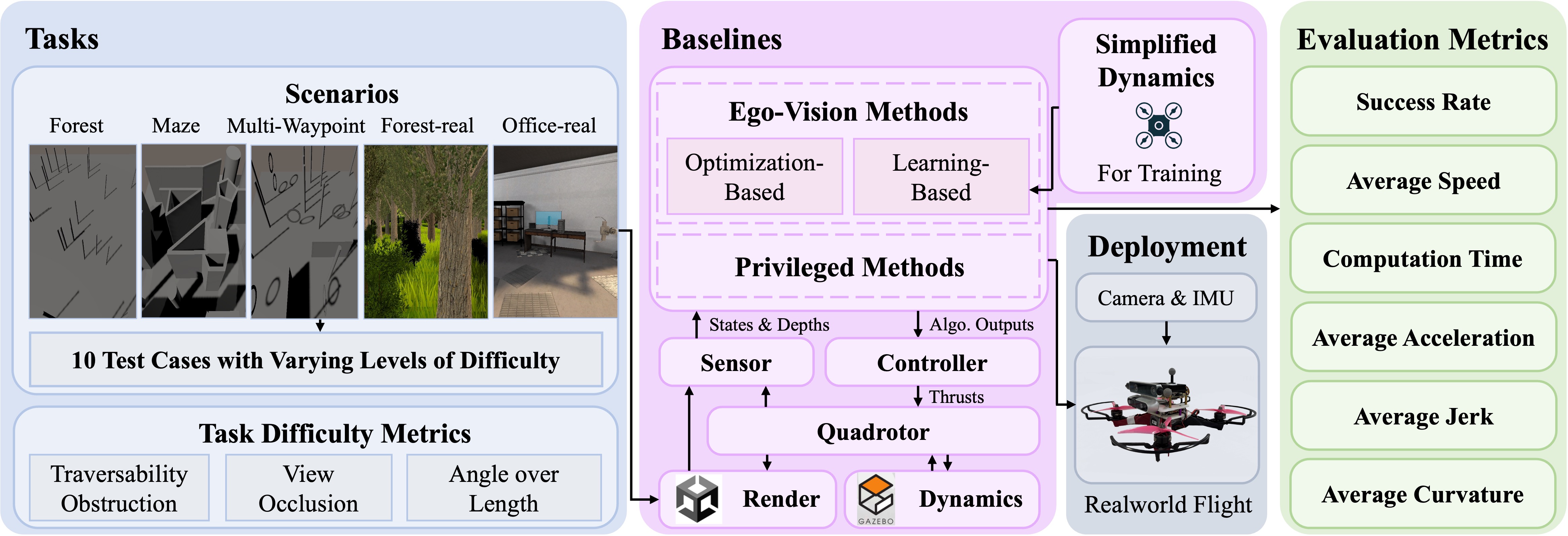
FlightBench is an unified open-source benchmark for planning methods on ego-vision-based navigation for quadrotors built on Flightmare. FlightBench provides cusomizable test scenarios (including three quantitative task difficulty metrics), representative planning algorithms, and comprehensive evaluation metrics. Here’s an overview of FlightBench.
| 📑Code | 📜 arXiv Paper | ⏩ Video. |
🔥News
[2025-03-01] 🚁 We have added Real-world Experiments. For demonstrations, please refer to our video.
[2025-03-01] 🏕️ We have added two more realistic environments. (See Scenarios. You can find the unity project here).
[2025-03-01] 📎 We have added a new learning-based baseline NPE (See our paper).
[2025-03-01] 💡 We have added more training details of learning-based methods to Implementation Details. The step-by-step tutorials for training the learning-based methods are available in Train Own Policy.
[2024-11-24] 🎁 We have added our full experimental results to Additional Simulation Results.
[2025-03-01] ⏩ We have added Summary Video with additional real-world experiments demos.
Table of Contents
- Introduction
- Table of Contents
- Installation
- Scenarios
- Let’s Fly
- Baselines
- Additional Simulation Results
- Real-world Experiments
- Citation
Installation
Before starting the installation, please add your ssh key to github.
Environment
- The installation is tested on Ubuntu-20.04
- An Nvidia GPU with installed drivers is necessary for rendering and RL training. CUDA>=11.1 is also necessary.
- ROS Noetic
- Gazebo 11
- Python 3.8. We recommend using python virtual environment. Use
sudo apt install python3-venvto install - gcc/g++ 9
Install FlightBench
Install the benchmark platform by the following commands:
mkdir flightbench_ws && cd flightbench_ws
mkdir src && cd src
sudo apt-get update && sudo apt-get install git cmake python3 python3-dev python3-venv python3-rosbag
git clone git@github.com:thu-uav/FlightBench.git
cd FlightBench
git submodule update --init --recursive

# Add FLIGHTMARE_PATH environment variable to .bashrc file:
echo "export FLIGHTMARE_PATH=path/to/FlightBench" >> ~/.bashrc
source ~/.bashrc

# We recommend using python virtual env to manage python packages
python3 -m venv flightpy # or any other name you like
source flightpy/bin/activate # active the venv

# install packages for training using pip
cd $FLIGHTMARE_PATH/flightrl
sudo apt-get install build-essential cmake libzmqpp-dev libopencv-dev libeigen3-dev
pip install -r requirements.txt
cd $FLIGHTMARE_PATH/flightlib

# install flightgym
pip install .

# install MAPPO
cd $FLIGHTMARE_PATH/flightrl
pip install -e .
Then install ROS part.
sudo apt-get update
export ROS_DISTRO=noetic
sudo apt-get install libgoogle-glog-dev protobuf-compiler ros-$ROS_DISTRO-octomap-msgs ros-$ROS_DISTRO-octomap-ros ros-$ROS_DISTRO-joy python3-vcstool python3-empy ros-$ROS_DISTRO-mavros
sudo pip install catkin-tools

# go flightbench_ws
cd flightbench_ws
catkin config --init --mkdirs --extend /opt/ros/$ROS_DISTRO --merge-devel --cmake-args -DPYTHON_EXECUTABLE=/usr/bin/python3 -DCMAKE_BUILD_TYPE=Release

catkin build
Install Baselines
# import benchmarks
cd src
vcs-import < FlightBench/flightbench/benchmarks.yaml

# install deps
sudo apt-get install libarmadillo-dev libglm-dev
# instsll nlopt
# go flightbench_ws
cd flightbench_ws
git clone https://github.com/stevengj/nlopt.git
cd nlopt
mkdir build
cd build
cmake ..
make
sudo make install
# install Open3d
cd flightbench_ws
git clone --recursive https://github.com/intel-isl/Open3D
cd Open3D
git checkout v0.9.0
git submodule update --init --recursive
./util/scripts/install-deps-ubuntu.sh
mkdir build
cd build
cmake -DCMAKE_INSTALL_PREFIX=/usr/local/bin/cmake ..
make -j$(nproc)
sudo make install

# compile baselines
cd flightbench_ws
catkin build
Install python packages for agile autonomy
# activate flightpy
source path/to/flightpy/bin/activate
cd path/to/benchmark_agile_autonomy
pip install -r requirements.txt
Install benchmark_sb_min_time
sudo apt-get install build-essential cmake pkg-config ccache zlib1g-dev libomp-dev libyaml-cpp-dev libhdf5-dev libgtest-dev liblz4-dev liblog4cxx-dev libeigen3-dev python3 python3-venv python3-dev python3-wheel python3-opengl
# into sb_min_time dir
cd benchmark_sb_min_time
git submodule update --init --recursive
make dependencies
make
Scenarios
Use Existing or Custom Scenarios
Use our scenarios
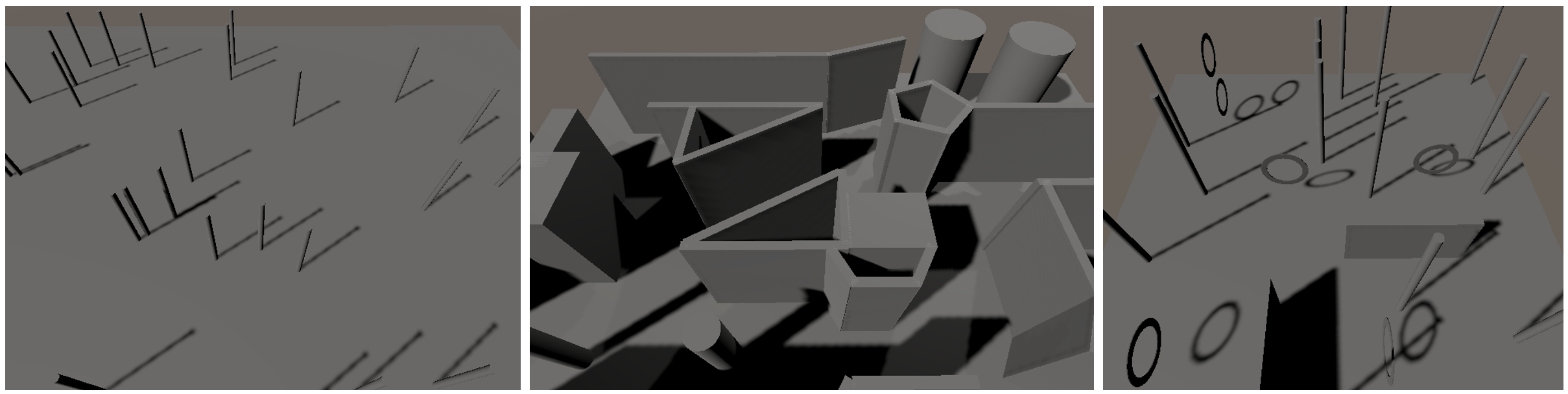
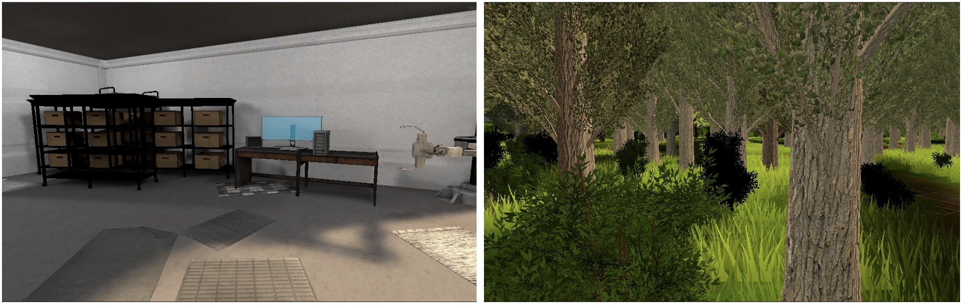
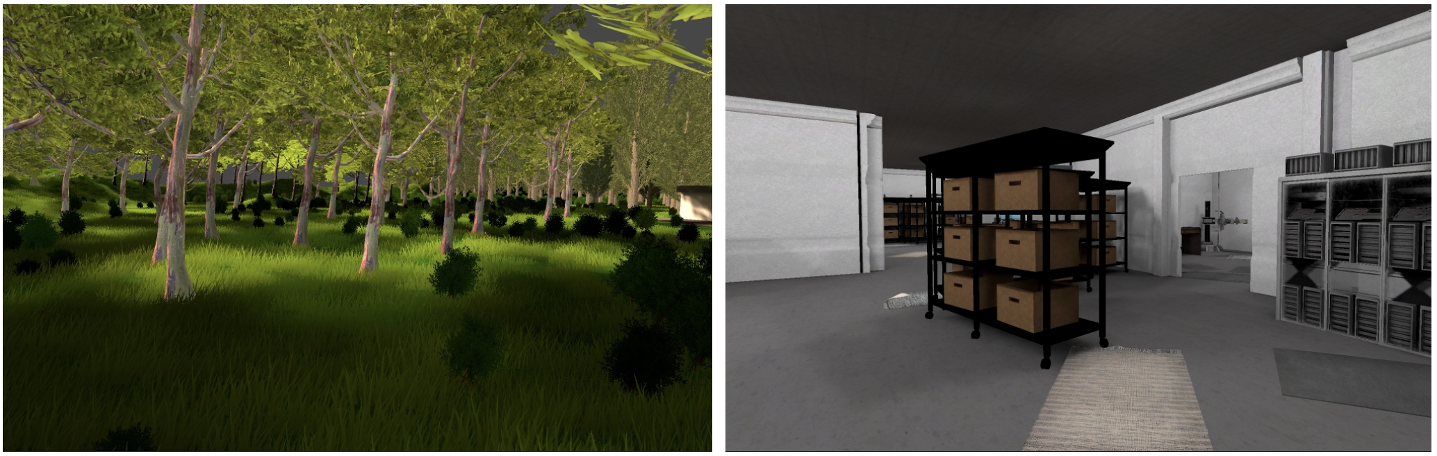
We provide 5 distinct scenarios: forest, maze, multi-waypoint, forest-real, and office-real. Forest-real and Office-real are photorealistic scenarios with testure and llighting condition. We provide outdoor natural lighting for Forest-real and indoor overhead lighting for Office-real.
- Download scene folder from here and put it to
path/to/FlightBench/sceneafter unzip. - Download render file from here. Put it into
path/to/FlightBench/flightrenderafter unzip.
Customize own scenarios
The Scenarios are customized using Unity. Our unity project is forked from flightmare_unity. You may choose to start with either flightmare_unity or our project for modifications.
- Install Unity hub following offical document
- Add a project, unity hub will automatically prompt whether to install unity editor (2020.1.10f1)
- Then you can edit and build the project following this
- Place the compiled files into
path/to/FlightBench/flightrender.
Based on Unity, the dynamic obstacles are also supported by scripting. For instance, add the following scripts to your obeject to enable an oribit move.
using System.Collections;
using System.Collections.Generic;
using UnityEngine;

public class orbit : MonoBehaviour
{
    public Transform target;
    public float speed = 2f;
    // Start is called before the first frame update
    void Start() {}
    // Update is called once per frame
    void Update()
    {
        Vector3 targetPos = target.position;
        Vector3 orbitPos = new Vector3(targetPos.x, transform.position.y, targetPos.z);
        Vector3 direction = (orbitPos - transform.position).normalized;
        float distanceToMove = speed * Time.deltaTime;
        Vector3 y = new Vector3(0, 1, 0);
        Vector3 newPosition = transform.position + Vector3.Cross(direction, y) * distanceToMove;
        transform.position = newPosition;
        transform.LookAt(targetPos);
    }
}
For training and evaluating RL-based methods, a scene folder should be organized as follow:
scene
|-- <scene_name_0>
|   |-- env.ply
|   |-- env-surface.ply
|   |-- roadmap_shortened_unique_path0_0.csv
|   |-- roadmap_shortened_unique_path1_0.csv
|   |-- roadmap_shortened_unique_pathn_0.csv
|
|-- <scene_name_1>
|   |-- env.ply
|   |-- env-surface.ply
|   |-- roadmap_shortened_unique_path0_0.csv
|   |-- roadmap_shortened_unique_path1_0.csv
|   |-- roadmap_shortened_unique_pathn_0.csv
|
|-- <scene_name_2>
|   ...
env.ply is the pointcloud file of the scenario, which can be generated by clicking the ‘scene save pointcloud’ bottom after compiling the unity project.
This section (Evaluate task difficulty) shows the generation of env-surface.ply and roadmap_shortened_unique_path.
Then put the folder into path/to/FlightBench/scene to support RL training and evluating.
Let’s Fly
Evaluate task difficulty
The task difficulty metrics defines on test cases. Each test case consists of a scenario, a start & end point, and a guiding path. The scenario, start point, and end point are self defined. We use path searching method from sb_min_time to generate guiding path.
According to the instructions of Fly sb_min_time, the topological guiding path will be generated at first step. Then move them into the origanized scene folder. Use the following command to generate the task difficulty value:
# activate flightpy venv
source path/to/flightpy/bin/activate
cd path/to/FlightBench/flightbench/scripts
python3 cal_difficulty.py scene/<scene_name>
# for example:
python3 cal_difficulty.py scene/maze-mid
We provide 8 test cases for evaluation.
| test_case_num | name | TO | VO | AOL |
|---|---|---|---|---|
| 0 | forest-low | 0.76 | 0.30 | 7.6e-4 |
| 1 | forest-mid | 0.92 | 0.44 | 1.6e-3 |
| 2 | forest-high | 0.9 | 0.6 | 5.7e-3 |
| 3 | maze-low | 1.42 | 0.51 | 1.4e-3 |
| 4 | maze-mid | 1.51 | 1.01 | 0.01 |
| 5 | maze-high | 1.54 | 1.39 | 0.61 |
| 6 | racing-low | 1.81 | 0.55 | 0.08 |
| 7 | racing-mid | 1.58 | 1.13 | 0.94 |
Fly with baseline algorithms
We integrate several representative planning algorithms in FlightBench, as detailed in the table below:
| No | baseline name | method type | code base |
|---|---|---|---|
| 1 | sb_min_time | privileged & sampling | https://github.com/uzh-rpg/sb_min_time_quadrotor_planning |
| 2 | fast_planner | Optimization-based | https://github.com/HKUST-Aerial-Robotics/Fast-Planner |
| 3 | ego_planner | Optimization-based | https://github.com/ZJU-FAST-Lab/ego-planner |
| 4 | tgk_planner | Optimization-based | https://github.com/ZJU-FAST-Lab/TGK-Planner |
| 5 | agile_autonomy | IL | https://github.com/uzh-rpg/agile_autonomy |
| 6 | learning_min_time | privileged & RL | / |
| 7 | learning_pa | RL + IL | / |
Fly sb_min_time
- Generate ESDF map from the pointcloud
cd path/to/bench_sb_min_time
# activate flightpy venv
source path/to/flightpy/bin/activate

# get surface first
python3 python/pcd_getsurface.py <pointcloud_path> <resolution>
# then generate ESDF
python3 python/map_pcd.py <pointcloud_path>
mv <pointcloud_path>.npy path/to/bench_sb_min_time/maps
- Generate trajectory
Then modify sst.yaml to set the map and waypoints. Run ./start.sh to generate trajectories.
- Start flying
Start simulator first
cd path/to/FlightBench/flightbench/scripts
./start_simulator.sh <test_case_num> <baseline_name>
Then start flying
# in another terminal
cd path/to/FlightBench/flightbench/scripts
./start_baseline.sh <test_case_num> <baseline_name>
Fly other baselines
We provide a unified test launch interface in start_simulator.sh and start_baseline.sh. Use the following commands to start a flight.
cd path/to/FlightBench/flightbench/scripts
./start_simulator.sh <test_case_num> <baseline_name>

#in another terminal
./start_baseline.sh <test_case_num> <baseline_name>
For learning-based methods, activating flightpy venv before start the baseline is needed.
Results
ROS bags will be saved automatically. Use the following command to parse the bag.
python3 bag_parser.py <bag_folder> <test_case_num> <baseline_name>
For conclusions and more details about our experiments, please refer to our paper
Baselines
Implementation Details
In this part, we detail the implementation specifics of baselines in FlightBench, focusing particularly on methods without open-source code.
Optimization-based Methods
Optimization-based methods typically employ a hierarchical structure, including an online mapping module followed by planning and control modules. Fast-Planner constructs both occupancy grid and Euclidean Signed Distance Field (ESDF) maps, whereas TGK-Planner and EGO-Planner only require an occupancy grid map. In the planning stage, EGO-Planner focuses on trajectory sections with new obstacles, acting as a local planner, while the other two use two-stage planning.
Fast-Planner, EGO-Planner, and TGK-Planner have all released open-source code. We integrate their open-source code into FlightBench and apply the same set of parameters for evaluation, as detailed bellow.
| Parameter | Value | Parameter | Value | |
|---|---|---|---|---|
| Max. Vel. | $ 3.0 ms^{-1}$ | Max. Acc. | $6.0 ms^{-2}$ | |
| All | Obstacle Inflation | $0.09$ | Depth Filter Tolerance | $0.15m$ |
| Map Resolution | $0.1m$ | |||
| Fast-Planner & TGK-Planner | krrt $\rho$ | $0.13 m$ | Replan Time | $0.005 s$ |
Learning-based Methods
Utilizing techniques such as imitation learning (IL) and reinforcement learning (RL), learning-based methods train neural networks for end-to-end planning, bypassing the time-consuming mapping process. The step-by-step tutorials for training these learning-based methods are available in Train Own Policy.
Agile
Agile employs DAgger to imitate an expert generating collision-free trajectories using Metropolis-Hastings sampling and outputs mid-level waypoints. Agile is an open-source learning-based baseline. The inputs and outputs of the network are defined as follows:
- input-state: shape: (18, ), range: [[-inf, inf]]. Contains goal direction, rotation matrix, linear & angular velocities of quadrotors. The goal direction is represented as a unit vector pointing to the position 5 seconds into the future.
- input-image: A depth image with a shape of (224, 224), which is encoded using MobileNet-V3.
- output: Represents ten future waypoints, with each waypoint containing x, y, z coordinates in body frame.
For each scenario, we finetune the policy from an open-source checkpoint using 100 rollouts. Following the approach described in benchmark_agile_autonomy/planner_learning/dagger_training, we use dagger to collect data online and train. All the data is annotated by experts using Metropolis-Hastings sampling.
LPA
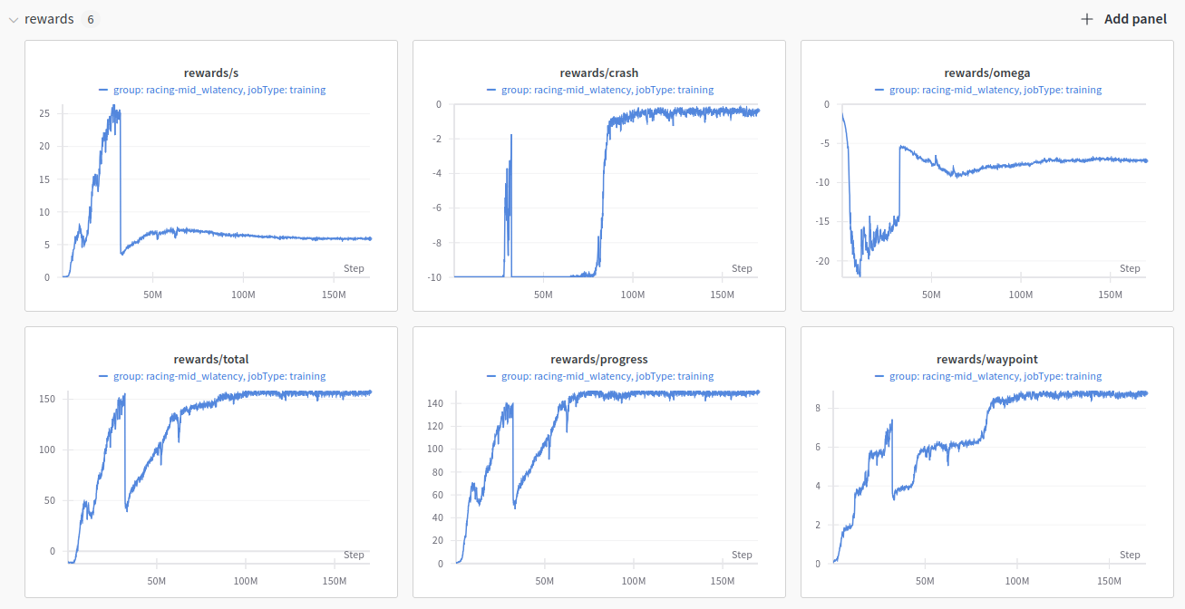
LPA combines IL and RL, starting with training a teacher policy using LMT, then distilling this expertise into a ego-vision-based student. LPA has not provided open-source code. Therefore, we reproduce the two stage training process based on their paper. The RL training stage involves adding a perception-aware reward to LMT method:
- Progress: Measured as the length of the flight trajectory projected onto the reference trajectory, in meters.
- Diff_Progress: The incremental progress achieved in a single training step.
- Waypoint: A bonus reward is given when the quadrotor passes a waypoint within a threshold, with the bonus depending on the distance to the waypoint.
- Crash: A penalty applied when the drone crashes.
- Omega: A penalty term defined as $-\omega^2$, which discourages aggressive actions.
-
Perception-Aware: A penalty term defined as $\exp(- \theta-\theta_{\text{dir}} )$, where $\theta$ and $\theta_{\text{dir}}$ refers to the yaw angle of the quadrotor and the reference trajectory.
Finally, a weighted sum of these rewards is calculated to determine the total reward.
PPO is used as the backbone algorithm. The algorithm is implemented in the folder onpolicy.algorithms.
At the IL stage, DAgger is employed to distill the teacher’s experience into an ego-vision student. The IL consists of two stages:
- Pretraining: We use the teacher policy to collect image data (See
onpolicy/scripts/collect_perception_aware_xxx.sh). With these data, pretrain the image encoder withonpolicy/runner/student_trainer.py. - DAgger Training: Freeze the image encoder and train the action network using
onpolicy/scripts/dagger_train_perception_aware.py.
Both teacher and student policies generate executable motion commands, specifically collective thrust and body rates (CTBR). All our experiments on LPA and LMT use the same set of hyperparameters, as listed after privileged methods.
Privileged Methods
SBMT
SBMT is an open-source sampling-based trajectory generator. Retaining the parameters in their paper, we use SBMT package to generate topological guide path to calculate the task difficulty metrics, and employ PAMPC to track the generated offline trajectories.
LMT
We reproduce LMT from scratch based on the original paper, implementing the observation, action, reward function, and training techniques described in the paper.
We give an example training environments in onpolicy.envs.learning_min_time.state_based_vec_env. The action and observation spaces are set as following:
- action space: shape: (4, ), range: [-inf, inf]. Then use tanh to map the input into [-1, 1], corresponding to the collective thrust and body rates. A PD controller is applied for tracking the desired command.
- obs space: shape: (13, ), range: [[-inf, inf]], containing position, orientation, linear & angular velocities of quadrotors.
The rewards are designed as follows:
- Progress: Measured as the length of the flight trajectory projected onto the reference trajectory, in meters.
- Diff_Progress: The incremental progress achieved in a single training step.
- Waypoint: A bonus reward is given when the quadrotor passes a waypoint within a threshold, with the bonus depending on the distance to the waypoint.
- Crash: A penalty applied when the drone crashes.
- Omega: A penalty term defined as $-\omega^2$, which discourages aggressive actions.
Finally, a weighted sum of these rewards is calculated to determine the total reward.
PPO is used as the backbone algorithm. The algorithm is implemented in the folder onpolicy.algorithms. Its hyperparameters are listed bellow.
| Parameter | Value | Parameter | Value | |
|---|---|---|---|---|
| Actor Lr | $5\times10^{-4}$ | Critic Lr | $5\times10^{-4}$ | |
| RL | PPO Epoch | $10$ | Batch Size | $51200$ |
| Max Grad. Norm. | $8.0$ | Clip Ratio | $0.2$ | |
| Entropy Coefficient | $0.01$ | |||
| IL(DAgger) | Lr | $2\times10^{-4}$ | Training Interval | $20$ |
| Training Epoch | $6$ | Max Episode | $2000$ |
System details
The overall system is implemented using ROS 1 Noetic Ninjemys. As mentioned in the main paper, we identify a quadrotor equipped with a depth camera and an IMU from real flight data. The physical characteristics of the quadrotor and its sensors are listed bellow.
| Parameter | Value | Parameter | Value | |
|---|---|---|---|---|
| Quadrotor | Mass | $1.0 kg$ | Max $\omega_{xy}$ | $8.0 rad/s$ |
| Moment of Inertia | $[5.9, 6.0, 9.8] g m^2$ | Max. $\omega_{z}$ | $3.0 rad/s$ | |
| Arm Length | $0.125 m$ | Max SRT | $0.1 N$ | |
| Torque Constant | $0.0178 m$ | Min. SRT | $5.0 N$ | |
| Sensors | Depth Range | $4.0 m$ | Depth FOV | $90^\circ\times 75^\circ$ |
| Depth Frame Rate | $30 Hz$ | IMU Rate | $100 Hz$ |
Train Own Policy
We use MAPPO to train the RL-related planning methods. Below, we will first introduce the simulation interface for training, followed by the training techniques for each method.
Perception & control interface
Perception data
RGBD image, odometry, and imu sensor data are provided. User can subscribe the following topics for flying.
/<quad_name>/ground_truth/odometry: pose and velocity (both linear and angular) under body frame/<quad_name>/ground_truth/imu: imu data, containing angular velocity and linear acceleration under body frame/<quad_name>/flight_pilot/rgb: a rgb8 encodingsensor_msgs.Imagemessage, containing the ego-vision rgb image./<quad_name>/flight_pilot/depth: a 32fc1 encodingsensor_msgs.Imagemessage, containing the ego-vision depth image.
Users can enable/disable the RGB and Depth topic separately by modifying path/to/FlightBench/flightros/params/default.yaml.
Control interface
There are many ways to control a quadrotor. At the lowest level, users can control the quadrotor using rate or attitude command.
- Topics for rate or attitude:
/<quad_name>/autopilot/control_command_input - Msg for rate or attitude:
quadrotor_msgs/ControlCommandWe provide a PD controller to track the desired rate or attitude. The parameters are available inpath/to/FlightBench/dep/quadrotor_control/simulation/rpg_rotors_interface/parameters/autopilot_air.yaml.
Higher level control commands are also supported by a MPC controller. The parameters are are available in path/to/FlightBench/dep/rpg_mpc/parameters/air.yaml.\
- Velocity contorl: when setting desired velocities, the quadrotor try tracking the target velocities. Send velocity commands (in
geometry_msgs/TwistStampedmsg) via topic/<quad_name>/autopilot/velocity_commandto enable velocity mode. - Full-state control: the message
quadrotor_msgs/TrajectoryPointsupports both linear and angular states up to 5th order. You can publish the target states with the desired timestamp using the message.
Training interface
FlightBench provides both state-based and image-based gym-like interfaces for RL training. We encourage users to use our environment as a code base to develop more RL algorithms & applications for drones.
We provide a gym-like base environment path/to/FlightBench/flightrl/onpolicy/envs/base_vec_env.py. Users can define their own training environment based on this.
State-based RL environment
We give an example onpolicy.envs.learning_min_time.state_based_vec_env.
- action space: shape: (4, ), range: [-inf, inf]. Then use tanh to map the input into [-1, 1], corresponding to the collective thrust and body rates. A PD controller is applied for tracking the desired command.
- obs space: shape: (13, ), range: [[-inf, inf]], containing position, orientation, linear & angular velocities of quadrotors.
Users can customize their own environment by modifying several functions like step, get_obs, and cal_reward.
Vision-based RL environment
Please refer to onpolicy.envs.learning_perception_aware.perception_aware_vec_env. We use a bridge, communicating with unity server, to get images.
The observation space could be set as a mixed dict:
obs_space_dict = {
    'imu': spaces.Box(low=np.float32(-np.inf), high=np.float32(np.inf),
                        shape=(self.args.state_len * self.n_imu, ),
                        dtype="float32"),
    'img': spaces.Box(low=0, high=256,
                        shape=(320, 240),
                        dtype="uint8"),
}
Train & eval learning_min_time policy
After installing flightgym and MAPPO, just activate flightpy venv and enter path/to/FlightBench/flightrl/onpolicy/scripts directory. Then use ./train_min_time_<scene_name>.sh to start training. The RL training process is logged using wandb.
Use ./train_min_time_<scene_name>.sh to evaluate the policy. Remember to change the ‘model_dir’ parameter in the .sh file to select which model to evaluate.
Feel free to adjust hyper-parameters in the .sh files!
Train & eval learning_perception_aware policy
Training a perception aware policy can be divided into two stages: RL + IL, while the IL stage consists of two steps.
- RL stage: use
./train_perception_aware_<scene_name>.shto train a state-based perception-aware teacher. - Pre-train stage: use
./collect_perception_aware_<scene_name>.shto collect data into the “offline_data” folder. Then usepython3 runner/studen_trainer.pyto pretrain the visual encoder and the action network. Before data collection, you need to startFM-full.x86_64(by double click) for rendering. - IL stage: use
dagger_train_pa_student_<scene_name>.shto train a vision-based student. We use DAgger to distill knowledge from the teach to the student. The training process will be logged using wandb. Key parameters are listed in the .sh files and .py files. Feel free to adjust them!
Then we can evaluate the student policy using the same way described in Fly with baseline algorithms.
- Modify the
model_dirparameter to choose your policy. - Use
start_simulatorandstart_baselineto start a flight, as discussed in Fly with baseline algorithms.
Refer to the reward curves if you train with our default settings.
Train agile_autonomy policy
We recommand creating another workspace and using their original pipeline to train an agile_autonomy policy. Due to differences in gcc version, training within this workspace may cause crashes.
Additional Simulation Results
Benchmarking Performance
Our paper analyzes the performance of the baselines only on the most challenging tests in each scenario due to space limitations. The full evaluation results are provided in the following three tables, represented in the form of mean(std).
Results in Forest
| Tests | Metric | SBMT | LMT | TGK | Fast | EGO | Agile | LPA |
|---|---|---|---|---|---|---|---|---|
| 1 | Success Rate $\uparrow$ | 0.90 | 1.00 | 1.00 | 1.00 | 1.00 | 1.00 | 1.00 |
| Avg. Spd. ($ms^{-1}$) $\uparrow$ |
17.90 (0.022) | 12.10 (0.063) | 2.329 (0.119) | 2.065 (0.223) | 2.492 (0.011) | 3.081 (0.008) | 11.55 (0.254) | |
| Avg. Curv. ($m^{-1}$) $\downarrow$ |
0.073 (0.011) | 0.061 (0.002) | 0.098 (0.026) | 0.100 (0.019) | 0.094 (0.010) | 0.325 (0.013) | 0.051 (0.094) | |
| Comp. Time ($ms$) $\downarrow$ |
2.477 (1.350)$\times 10^{5}$ | 2.721 (0.127) | 11.12 (1.723) | 7.776 (0.259) | 3.268 (0.130) | 5.556 (0.136) | 1.407 (0.036) | |
| Avg. Acc. ($ms^{-3}$) $\downarrow$ |
31.54 (0.663) | 9.099 (0.321) | 0.198 (0.070) | 0.254 (0.054) | 54.97 (0.199) | 4.934 (0.385) | 10.89 (0.412) | |
| Avg. Jerk ($ms^{-5}$) $\downarrow$ |
4644 (983.6) | 6150 (189.2) | 0.584 (0.216) | 3.462 (1.370) | 3.504 (24.048) | 601.3 (48.63) | 7134 (497.2) | |
| 2 | Success Rate $\uparrow$ | 0.80 | 1.00 | 1.00 | 1.00 | 1.00 | 1.00 | 1.00 |
| Avg. Spd. ($ms^{-1}$) $\uparrow$ |
14.99 (0.486) | 11.68 (0.072) | 2.300 (0.096) | 2.672 (0.396) | 2.484 (0.008) | 3.059 (0.006) | 9.737 (0.449) | |
| Avg. Curv. ($m^{-1}$) $\downarrow$ |
0.069 (0.004) | 0.066 (0.001) | 0.116 (0.028) | 0.068 (0.035) | 0.122 (0.006) | 0.327 (0.025) | 0.071 (0.038) | |
| Comp. Time ($ms$) $\downarrow$ |
2.366 (2.009)$\times 10^{5}$ | 2.707 (0.079) | 11.75 (1.800) | 7.618 (0.220) | 3.331 (0.035) | 5.541 (0.173) | 1.411 (0.036) | |
| Avg. Acc. ($ms^{-3}$) $\downarrow$ |
34.88 (1.224) | 11.14 (0.296) | 0.117 (0.084) | 0.258 (0.148) | 1.265 (0.178) | 4.703 (0.876) | 14.79 (0.564) | |
| Avg. Jerk ($ms^{-5}$) $\downarrow$ |
4176 (1654) | 9294 (380.7) | 0.497 (0.484) | 4.017 (1.471) | 83.96 (20.74) | 751.8 (118.4) | 11788 (803.5) | |
| 3 | Success Rate $\uparrow$ | 0.80 | 1.00 | 0.90 | 0.90 | 1.00 | 0.90 | 1.00 |
| Avg. Spd. ($ms^{-1}$) $\uparrow$ |
15.25 (2.002) | 11.84 (0.015) | 2.300 (0.100) | 2.468 (0.232) | 2.490 (0.006) | 3.058 (0.008) | 8.958 (0.544) | |
| Avg. Curv. ($m^{-1}$) $\downarrow$ |
0.065 (0.017) | 0.075 (0.001) | 0.078 (0.035) | 0.059 (0.027) | 0.082 (0.013) | 0.367 (0.014) | 0.080 (0.094) | |
| Comp. Time ($ms$) $\downarrow$ |
2.512 (0.985)$\times 10^{5}$ | 2.792 (0.168) | 11.54 (1.807) | 7.312 (0.358) | 3.268 (0.188) | 5.614 (0.121) | 1.394 (0.039) | |
| Avg. Acc. ($ms^{-3}$) $\downarrow$ |
28.39 (3.497) | 10.29 (0.103) | 0.249 (0.096) | 0.192 (0.119) | 0.825 (0.227) | 4.928 (0.346) | 9.962 (0.593) | |
| Avg. Jerk ($ms^{-5}$) $\downarrow$ |
4270 (1378) | 8141 (133.2) | 1.030 (0.609) | 3.978 (1.323) | 58.395 (15.647) | 937.0 (239.2) | 11352 (693.6) |
Results in Maze
| Tests | Metric | SBMT | LMT | TGK | Fast | EGO | Agile | LPA |
|---|---|---|---|---|---|---|---|---|
| 1 | Success Rate $\uparrow$ | 0.80 | 1.00 | 0.90 | 1.00 | 0.90 | 1.00 | 0.80 |
| Avg. Spd. ($ms^{-1}$) $\uparrow$ |
13.66 (1.304) | 10.78 (0.056) | 2.251 (0.123) | 2.097 (0.336) | 2.022 (0.010) | 3.031 (0.004) | 5.390 (0.394) | |
| Avg. Curv. ($m^{-1}$) $\downarrow$ |
0.087 (0.025) | 0.079 (0.002) | 0.154 (0.049) | 0.113 (0.029) | 0.179 (0.011) | 0.135 (0.010) | 0.252 (0.084) | |
| Comp. Time ($ms$) $\downarrow$ |
1.945 (0.724)$\times 10^{5}$ | 2.800 (0.146) | 11.76 (0.689) | 7.394 (0.475) | 3.053 (0.035) | 5.535 (0.140) | 1.369 (0.033) | |
| Avg. Acc. ($ms^{-3}$) $\downarrow$ |
34.57 (6.858) | 13.26 (0.374) | 0.277 (0.161) | 0.392 (0.223) | 1.599 (0.220) | 1.023 (0.128) | 18.17 (0.708) | |
| Avg. Jerk ($ms^{-5}$) $\downarrow$ |
4686 (1676) | 10785 (149.1) | 0.809 (0.756) | 3.716 (1.592) | 109.2 (25.81) | 65.94 (15.66) | 8885 (206.4) | |
| 2 | Success Rate $\uparrow$ | 0.70 | 1.00 | 0.80 | 0.90 | 0.60 | 0.70 | 0.80 |
| Avg. Spd. ($ms^{-1}$) $\uparrow$ |
13.67 (0.580) | 10.57 (0.073) | 2.000 (0.065) | 2.055 (0.227) | 2.022 (0.001) | 3.052 (0.003) | 9.314 (0.168) | |
| Avg. Curv. ($m^{-1}$) $\downarrow$ |
0.082 (0.009) | 0.088 (0.002) | 0.157 (0.053) | 0.090 (0.026) | 0.109 (0.002) | 0.193 (0.009) | 0.076 (0.081) | |
| Comp. Time ($ms$) $\downarrow$ |
2.188 (1.160)$\times 10^{5}$ | 3.047 (0.196) | 11.58 (0.514) | 7.557 (0.283) | 2.997 (0.022) | 5.579 (0.102) | 1.371 (0.037) | |
| Avg. Acc. ($ms^{-3}$) $\downarrow$ |
31.68 (1.443) | 15.99 (0.274) | 0.252 (0.102) | 0.278 (0.084) | 1.090 (0.147) | 1.772 (0.336) | 10.89 (0.531) | |
| Avg. Jerk ($ms^{-5}$) $\downarrow$ |
2865 (566.8) | 8486 (392.6) | 0.967 (0.759) | 3.999 (1.015) | 103.2 (18.75) | 171.4 (30.66) | 2062 (190.4) | |
| 3 | Success Rate $\uparrow$ | 0.60 | 0.90 | 0.50 | 0.60 | 0.20 | 0.50 | 0.50 |
| Avg. Spd. ($ms^{-1}$) $\uparrow$ |
8.727 (0.168) | 9.616 (0.112) | 1.849 (0.120) | 1.991 (0.134) | 2.189 (0.167) | 2.996 (0.012) | 8.350 (0.286) | |
| Avg. Curv. ($m^{-1}$) $\downarrow$ |
0.313 (0.034) | 0.134 (0.008) | 0.168 (0.060) | 0.229 (0.057) | 0.332 (0.020) | 0.682 (0.084) | 0.214 (0.093) | |
| Comp. Time ($ms$) $\downarrow$ |
1.649 (1.539)$\times 10^{5}$ | 2.639 (0.100) | 10.29 (0.614) | 8.918 (0.427) | 3.552 (0.111) | 5.469 (0.081) | 1.422 (0.037) | |
| Avg. Acc. ($ms^{-3}$) $\downarrow$ |
60.73 (5.686) | 26.26 (1.680) | 0.500 (0.096) | 0.786 (0.306) | 1.910 (0.169) | 15.45 (3.368) | 37.30 (1.210) | |
| Avg. Jerk ($ms^{-5}$) $\downarrow$ |
6602 (685.1) | 4649 (305.8) | 6.740 (0.226) | 9.615 (4.517) | 80.54 (7.024) | 2151 (470.2) | 4638 (428.4) |
Results in Multi-Waypoint(MW)
| Tests | Metric | SBMT | LMT | TGK | Fast | EGO | Agile | LPA |
|---|---|---|---|---|---|---|---|---|
| 1 | Success Rate $\uparrow$ | 0.60 | 0.90 | 0.90 | 1.00 | 1.00 | 1.00 | 0.80 |
| Avg. Spd. ($ms^{-1}$) $\uparrow$ |
10.13 (0.343) | 11.06 (0.107) | 1.723 (0.075) | 2.164 (0.140) | 2.512 (0.017) | 3.017 (0.029) | 8.216 (1.459) | |
| Avg. Curv. ($m^{-1}$) $\downarrow$ |
0.177 (0.027) | 0.087 (0.004) | 0.119 (0.045) | 0.118 (0.017) | 0.159 (0.012) | 0.406 (0.048) | 0.223 (0.035) | |
| Comp. Time ($ms$) $\downarrow$ |
1.199 (0.371)$\times 10^{5}$ | 2.834 (0.163) | 15.32 (0.684) | 9.265 (0.542) | 3.464 (8.786) | 5.610 (0.161) | 1.393 (0.035) | |
| Avg. Acc. ($ms^{-3}$) $\downarrow$ |
46.98 (10.46) | 19.67 (1.300) | 0.540 (0.080) | 0.533 (0.169) | 1.063 (0.173) | 7.456 (1.249) | 34.00 (1.551) | |
| Avg. Jerk ($ms^{-5}$) $\downarrow$ |
5051 (865.4) | 5641 (358.0) | 6.287 (0.899) | 12.03 (4.145) | 64.50 (12.90) | 1378 (776.3) | 9258 (2238) | |
| 2 | Success Rate $\uparrow$ | 0.70 | 0.90 | 0.40 | 0.80 | 0.50 | 0.60 | 0.50 |
| Avg. Spd. ($ms^{-1}$) $\uparrow$ |
5.587 (1.351) | 6.880 (0.366) | 1.481 (0.092) | 1.735 (0.241) | 2.132 (0.339) | 3.053 (0.034) | 6.721 (0.980) | |
| Avg. Curv. ($m^{-1}$) $\downarrow$ |
0.469 (0.029) | 0.296 (0.031) | 0.463 (0.046) | 0.320 (0.047) | 0.617 (0.216) | 0.668 (0.056) | 0.263 (0.051) | |
| Comp. Time ($ms$) $\downarrow$ |
6.437 (0.250)$\times 10^{5}$ | 2.649 (0.185) | 12.32 (2.042) | 9.725 (0.818) | 4.584 (0.734) | 5.683 (0.140) | 1.390 (0.039) | |
| Avg. Acc. ($ms^{-3}$) $\downarrow$ |
80.95 (15.10) | 31.23 (1.213) | 1.067 (0.083) | 0.972 (0.470) | 5.060 (1.523) | 16.86 (1.422) | 36.77 (10.36) | |
| Avg. Jerk ($ms^{-5}$) $\downarrow$ |
9760 (1000) | 16565 (3269) | 25.52 (7.914) | 22.72 (11.14) | 155.8 (114.1) | 2070 (551.0) | 6187 (956.2) |
The results indicate that optimization-based methods excel in energy efficiency and trajectory smoothness. In contrast, learning-based approaches tend to adopt more aggressive maneuvers. Although this aggressiveness grants learning-based methods greater agility, it also raises the risk of losing balance in sharp turns.
Failure Cases
As discussed in our paper, our benchmark remains challenging for ego-vision planning methods. In this part, we specifically examine the most demanding tests within the Maze and Multi-Waypoint scenarios to explore how scenarios with high VO and AOL cause failures. Video illustrations of failure cases are provided in the supplementary material.
As shown bellow (Left), Test 3 in the Maze scenario has the highest VO among all tests. Before the quadrotor reaches waypoint 1, its field of view is obstructed by wall (A), making walls (B) and the target space (C) invisible. The sudden appearance of wall (B) often leads to collisions. Additionally, occlusions caused by walls (A) and (C) increase the likelihood of navigating to a local optimum, preventing effective planning towards the target space (C).
The figure bellow (Right) illustrates a typical Multi-Waypoint scenario characterized by high VO, TO, and AOL. In this scenario, the quadrotor makes a sharp turn at waypoint 2 while navigating through the waypoints sequentially. The nearest obstacle, column (D), poses a significant challenge due to the need for sudden reactions. Additionally, wall (E), situated close to column (D), often leads to crashes for baselines with limited real-time replanning capabilities.

Maze Scenario

MW Scenario
Analyses on Effectiveness of Different Metrics
Correlation Calculation Method.
As the value of two metrics to be calculated for the correlation coefficient are denoted as ${x_i},\ {y_i}$, respectively. The correlation coefficient between ${x_i}$ and ${y_i}$ defines as
\[ \text{Corr}_{x,y} = \frac{\sum_i (x_i-\bar x)(y_i - \bar y)}{\sqrt{\sum_i (x_i-\bar x)^2\sum (y_i-\bar y)^2}}, \]
where $\bar x,\ \bar y$ are the average values of ${x_i}$ and ${y_i}$.
Results
Figures bellow shows the correlation coefficients between six performance metrics and three difficulty metrics for each method across multiple scenarios. As analyzed in our paper, TO and AOL significantly impact the motion performance of two privileged methods (SBMT and LMT). In scenarios with high TO and AOL, the baselines tend to fly slower, consume more energy, and exhibit less smoothness. Ego-vision methods are notably influenced by partial perception, making VO a crucial factor. Consequently, high VO greatly decreases the success rate of ego-vision methods, much more so than it does for privileged methods.
When comparing the computation times of different methods, we observe that the time required by learning-based methods primarily depends on the network architecture and is minimally influenced by the scenario. Conversely, the computation times for optimization- and sampling-based methods are affected by both AOL and TO. Scenarios with higher TO and AOL demonstrate increased planning complexity, resulting in longer computation times.

Correlations for SBMT

Correlations for LMT

Correlations for TGK-Planner

Correlations for LMT

Correlations for EGO-Planner

Correlations for Agile

Correlations for LPA
Real-world Experiments
EGO and Agile are selected for real-world validation. We use our customized quadrotor for deployment. Our quadrotor integrates an NVIDIA Orin NX for computation and utilizes MAVLink to interface with the PX4 flight controller for low-level control.

Full-Pipeline Experiment
We first conduct full-pipeline flight to show the deployment capability. All state estimation, computation, and control are performed on board. The flying trajectories are as follow:
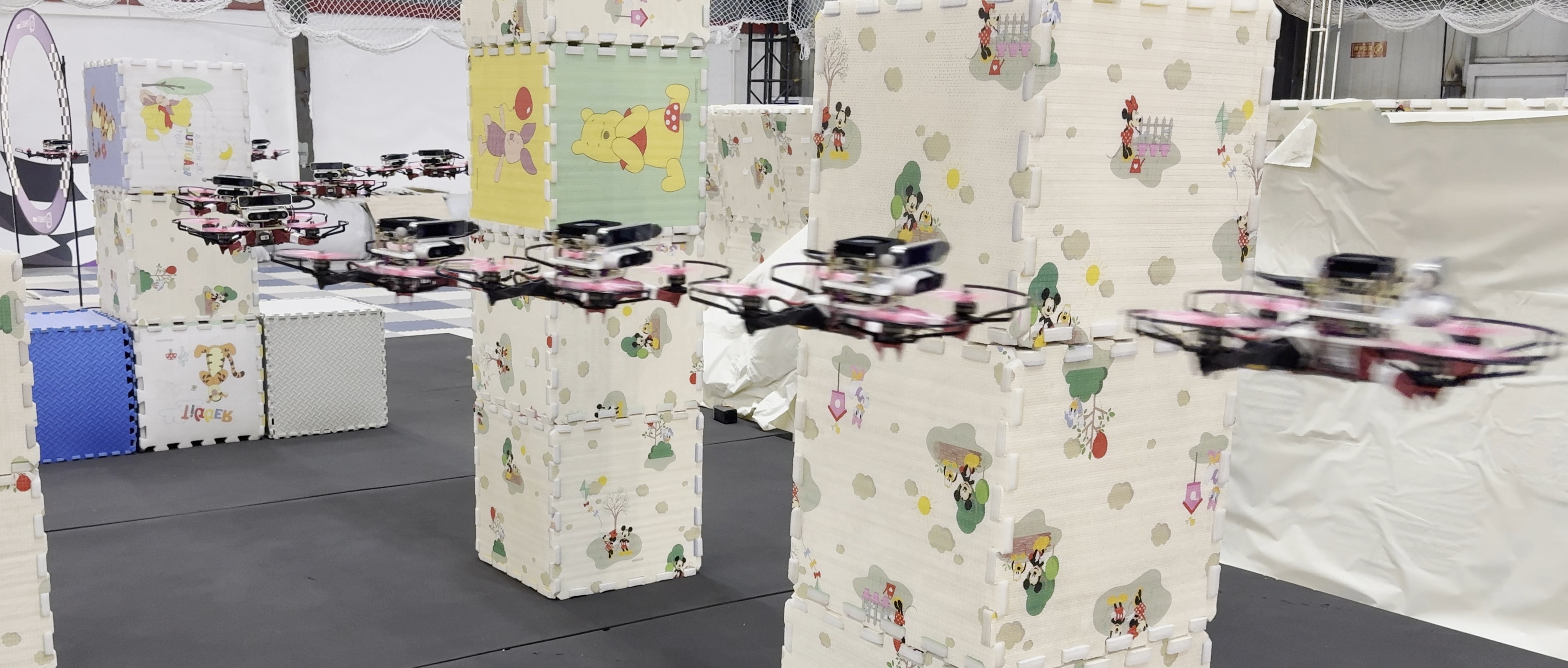
Get more demonstrations through our video.
Hardware-In-The-Loop Experiments
The data pipeline of hardware-in-the-loop(HITL) experiment is shown in the figure below. The quadrotor flies in an empty space, while getting image perception from the simulator. We use swarm ros bridge for data communication via WLAN.

Using HITL experiment, we can quantitatively analyze the real-world flight performance.
| Tests | TO | VO | AOL | EGO | Agile | ||||||
|---|---|---|---|---|---|---|---|---|---|---|---|
| Avg. Spd. ($ms^{-1}$) $\uparrow$ |
Avg. Curv. ($m^{-1}$) $\downarrow$ |
Avg. Acc. ($ms^{-3}$) $\downarrow$ |
Avg. Jerk ($ms^{-5}$) $\downarrow$ |
Avg. Spd. ($ms^{-1}$) $\uparrow$ |
Avg. Curv. ($m^{-1}$) $\downarrow$ |
Avg. Acc. ($ms^{-3}$) $\downarrow$ |
Avg. Jerk ($ms^{-5}$) $\downarrow$ |
||||
| 1 | 0.98 | 0.57 | 3$\times 10^{-4}$ | 1.39 | 0.54 | 1.40 | 4.85$\times 10^2$ | 1.45 | 0.65 | 2.11 | 3.99$\times 10^3$ |
| 2 | 1.81 | 1.82 | 0.027 | 1.32 | 0.92 | 1.68 | 5.64$\times 10^2$ | 1.47 | 1.61 | 5.62 | 6.64$\times 10^3$ |
| 3 | 2.07 | 1.85 | 0.040 | 1.39 | 1.55 | 5.20 | 7.70$\times 10^2$ | 1.51 | 1.62 | 7.82 | 8.36 $\times 10^3$ |
In more challenging scenarios (with higher TO, VO, and AOL), the quadrotor exhibits increased curvature, acceleration, and jerk during the flight. In the same scenarios, Agile shows larger curvature, acceleration, and jerk compared to EGO, leading to less smooth flight.
Citation
Please cite our paper if you use FlightBench in your work.
@article{yu2024flightbench,
  title={FlightBench: Benchmarking Learning-based Methods for Ego-vision-based Quadrotors Navigation},
  author={Yu, Shu-Ang and Yu, Chao and Gao, Feng and Wu, Yi and Wang, Yu},
  journal={arXiv preprint arXiv:2406.05687},
  year={2024}
}